 Shai Greenberg
How to load pandemic reports of COVID-19, the virus that is spreading in an unbelievable rate throughout the world, into Elasticsearch and get them ready to be visualized in Kibana.
The novel Coronavirus, also known as COVID-19, is spreading at an unbelievable rate throughout the world. This can lead to confusion and fright especially since the media usually doesn't deliver news in a scientific way. Lucky for us (well, under the circumstances), official pandemic reports datasets are available on the internet, and those datasets can be used to better understand the nature of this disease. You don’t have to be a data scientist to get a basic grasp of the relevant statistics - keep reading to learn how to do so.
Kibana and Elasticsearch offer a good way to quickly create visualizations based on datasets. Even if you don't have Elasticsearch and Kibana as part of your landscape, you can quickly set them up locally and play around with a CSV or a JSON-formatted dataset in no time.
In this post series we will go over a short tutorial for doing just that, and you can follow along. Kibana requires running an Elasticsearch instance however, for the purposes of this blog, we won't dive into Elasticsearch too much, but rather install both and focus on the data discovery perspective.
Setup
To follow along this series you should have Elasticsearch and Kibana running. If you don't have a Kibana instance to work on, the easiest way to launch them you is by using Docker. You can use our docker-compose setup here. Download it and run docker-compose up to get started. Alternatively, you can get the binaries from the official website here.
Once you have launched Elasticsearch and Kibana, you should be able access Kibana at http://localhost:5601 . The following sections assume Elasticsearch and Kibana versions 7.6, but the functionality described exists, though under other names, in earlier versions as well.
Loading the dataset
The dataset we will use details the number of cases, deaths and recoveries by countries and states, and has daily updates which we can use to also show this info on the time axis. The data is being collected by the Johns Hopkins University Center for Systems Science and Engineering. The dataset is located here.
You can see the data is divided into daily files. There's actually also a file that aggregates data from all days so far, but loading that file would actually require some pre-processing that is out of the scope at the moment. For now, we will focus on loading a single file at a time to start with an initial exploration. Go ahead and get one or more of the files from the dataset (by downloading it in its entirety, or getting the file from the "raw" link in the file page). Update: As the schema used in new files is different than the one referred to in this post, It is best to use files from the period between March 1st 2020 and March 21st. We'll discuss how to make future files compatible to this post in another post.
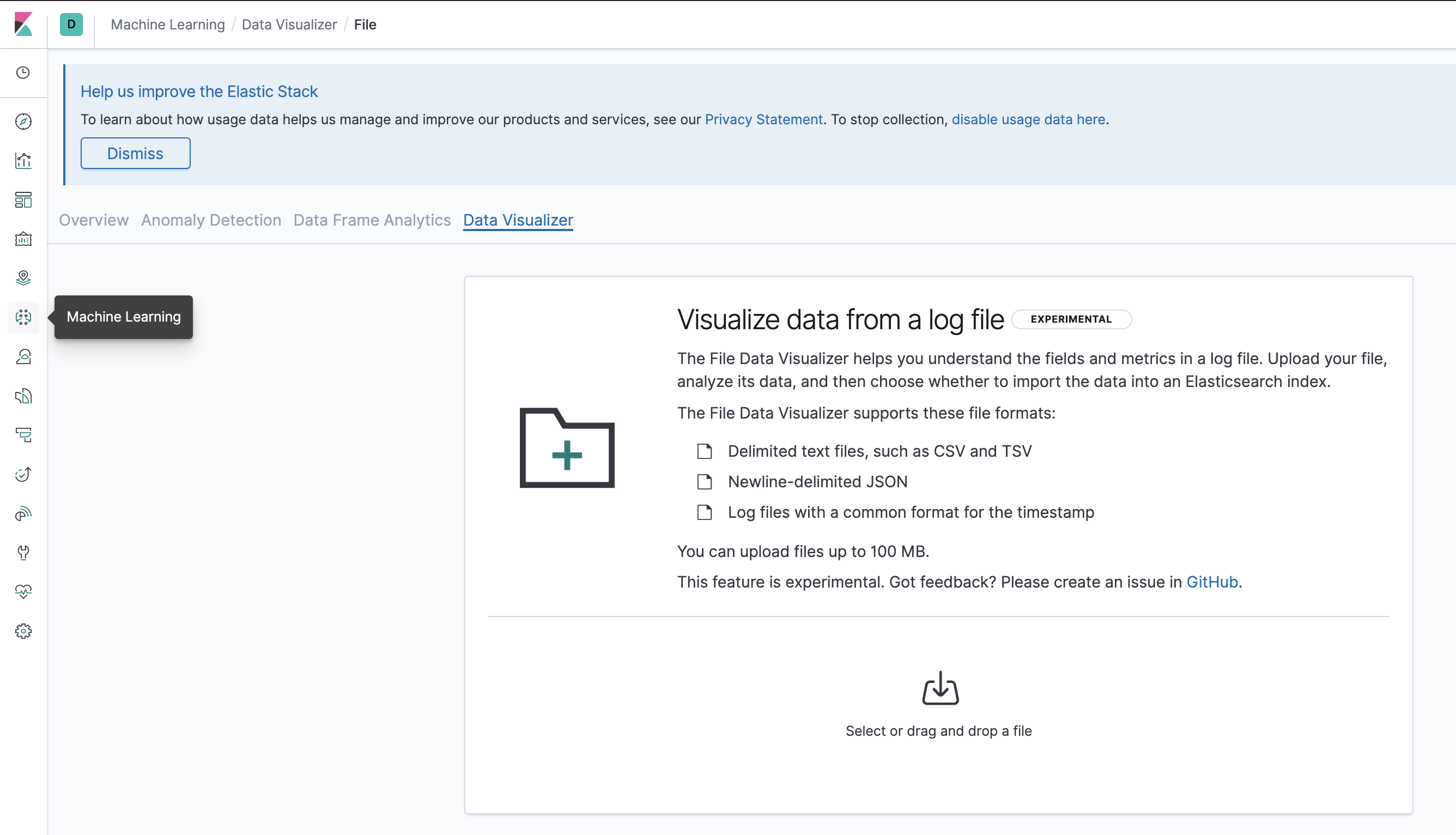
In order to load the file into Elasticsearch, go to Kibana's Machine Learning application, and under "Import Data" choose "Upload File". Go ahead and choose one of the files you've downloaded.
Kibana's Import Data mechanism is a simple interface to load a file into an Elasticsearch index, as well as optionally creating an Index Pattern in Kibana. In general terms, an index is where you store the data and an index pattern is a logical layer created to view it. The mechanism also allows for simple pre-processing tasks meant to transform and enrich the data, which we'll have to do in order to slice the data based on time and view it using a map.
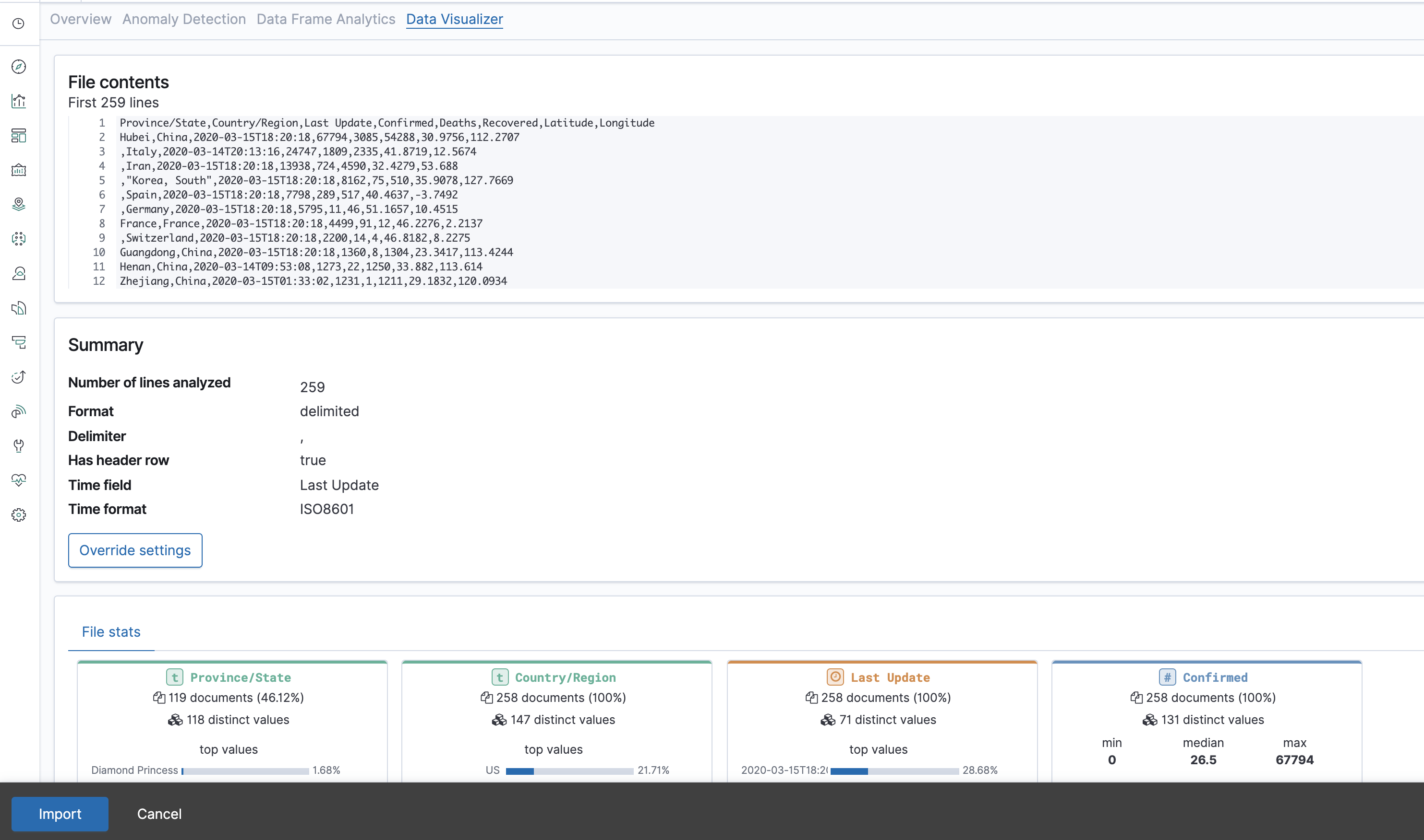
After uploading the file you'll see a screen that displays the file's contents, allows overriding the way the file is read, and shows stats on the columns in the file. This is a nice way to familiarize yourself with the data, if you haven't yet. Hurrah, Looks like we are already visualizing the data, and that's before we've even loaded it!
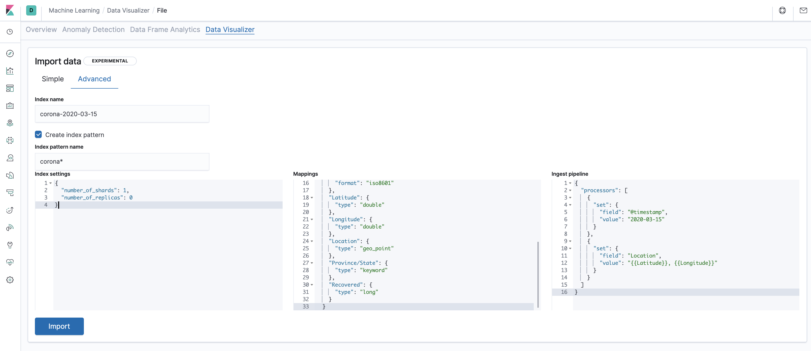
Hit the import button. In the next screen you'll be asked to provide the index name. However, we're going to do a bit more than that. Click the "Advanced" tab. You now get several inputs, and we'll go over each one providing the required syntax for the file and explaining what that input does.
-
"Index name" is where you want the data to be loaded. Optimally Elasticsearch indices can be pretty large and probably all of the data for the purposes of this example can use one index. However the upload interface doesn't allow to upload several files into one index. Instead, we'll create several indices with a certain naming convention, and view all of them by using the index pattern. One conventional naming pattern would be corona-YYYY-MM-DD, so let's use that - if we've used the file
03-15-2020.csv, the index name would becorona-2020-03-15.The index pattern name would have to match every additional index we create. So, we'll call itcorona*(sans quotes). -
Index settings are based on the architecture of your Elasticsearch, and the default setting isn't necessarily relevant to you, especially if you've installed Kibana/ES locally. Instead, let's use the following:
{ "number_of_shards": 1, "number_of_replicas": 0 } -
Mapping is a pretty wide concept in Elasticsearch but, for simplicity sake, let's just say it's the way the search data in Elasticsearch is structured. Here we'll also need to change the default a bit, and use the following:
{ "@timestamp": { "type": "date" }, "Confirmed": { "type": "long" }, "Country/Region": { "type": "keyword" }, "Deaths": { "type": "long" }, "Last Update": { "type": "date", "format": "iso8601" }, "Latitude": { "type": "double" }, "Longitude": { "type": "double" }, "Location": { "type": "geo_point" }, "Province/State": { "type": "keyword" }, "Recovered": { "type": "long" } } -
Finally, the ingest pipeline is a transformation that's done on the data before inserting it into Elasticsearch. Again, we'll use code designed to handle the input files rather than the default:
{
  "processors": [
    {
      "set": {
        "field": "@timestamp",
        "value": "2020-03-15"
      }
    },
    {
      "set": {
        "field": "Location",
        "value": "{{Latitude}}, {{Longitude}}"
      }
    }
  ]
}
Click Import and the data will be imported. Below you'll get options to view the data in the data visualizer, which is similar to the preview from before, only with a bit more visualizations. After that, feel free to click the Data Visualizer tab at the top of the screen again and import additional files.
Notice that for any additional files you'll have to change the index name and the value for @timestamp in the processor. Additionally, you won't need to create the index pattern as we've already created it (but remember that the index name should match the pattern corona*).
Playing around with Discover
Kibana's most basic data exploration tool is called Discover. It is essentially a customizable table view that lets you explore the data with filters, column selection and a simple chart.
Let's start by changing the time filter to show data from the correct period. Click the time filter at the top right of the screen, choose "Relative" and then choose a time period which contains the data you have loaded, and then refresh. You'll be able to see the data you've inserted both in a chart preview and in a table preview.
The chart shows the document count for each day, which is essentially the number of reports from different places per day (as Elasticsearch has a document store, a "record" from the file becomes a"document" in Elasticsearch). While the count is not a meaningful statistic, this immediately helps you see which days fall into the filter period.
The table shows the actual data: here you can see a clear view of each document, and you can also click to expand, near the document, to see either its fields arranged in a table or the actual document saved in Elasticsearch in JSON format.
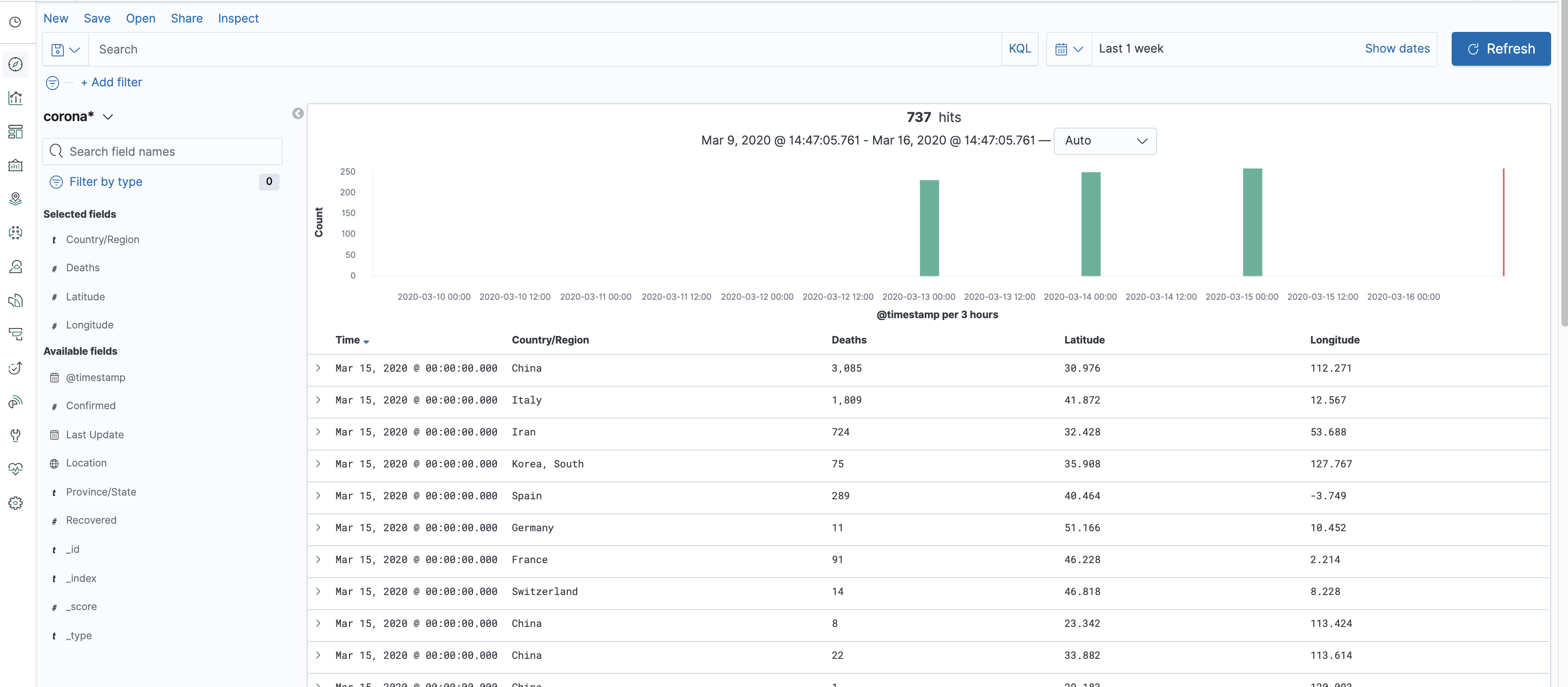
You can choose to view more or fewer columns in the table by using the pivot-like field selector on the left side of the screen. Clicking each field in that selection will also give you the top values for it, and allow you to jump into visualization mode, but that’s something we’ll go into in the next post.
Finally, you also have an option to add filters that are not time-based in the top left side of the screen, and even do a text search on all of the fields.
After exploring with Discover to your satisfaction, you can save your search in order to be able to return to it at a later time - you’ll see a save button at the top and there’s also an open button. Saving your search will allow you to get back to where you last stopped; and better yet, to create visualizations based on data from your searches. More on that later.
Next up
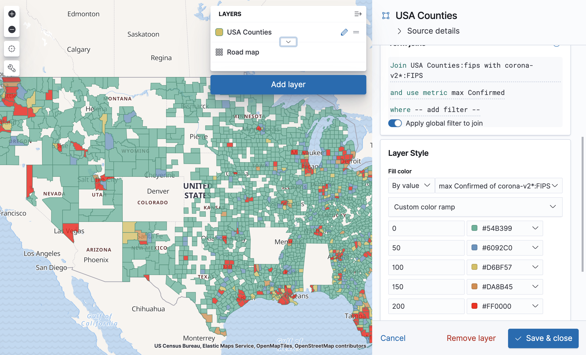
In the next post in this series, we create Kibana visualizations and add them to an impressive Dashboard, which shows the spread of COVID-19 around the world.
We will also look at more advanced Kibana and Elasticsearch features and applications in future posts. Stay tuned!
Need help setting up Elasticsearch and Kibana for your use case? Reach out to us today!


Comments are now closed