Tuning Elasticsearch: Garbage Collection Algorithms

In this series of articles we look at levers and toggles that are used for tuning your Elasticsearch cluster, and discuss how to find the optimum values. In this article, we will discuss garbage collection algorithms, and which one to use.

In the previous post we discussed how a correctly sized heap size can have a huge impact on the overall query performance of Elasticsearch.

Garbage collection frequency is more nuanced. On one hand, a smaller heap results in more frequent garbage collections. If responding to a single query requires Elasticsearch to run the garbage collector multiple times, it can severely degrade the performance of the cluster. On the other hand, a larger heap means that each garbage collection takes longer, and these longer pauses can also lead to reduced performance.

Correctly sized caches can have a huge impact on the overall query performance, as well as Elasticsearch cluster stability.

Garbage Collection Algorithms

Java has experimented with several different garbage collection algorithms over the years, and with modern versions there are 2 algorithms which are relevant to Elasticsearch: parallel and garbage-first (G1).

If you're already familiar with Java garbage collection, you may have heard of concurrent-mark-and-sweep (CMS), but in Java 14 it's been removed in favor of the G1 GC.

There are many great articles that go into the details of how these garbage collection algorithms work, and going into the details is beyond the scope of this article. What we'll look at today is why you might want to choose one algorithm over the other. To put the bottom line up front: you should benchmark on your actual workload, because the two methods can have very different performance characteristics with only slight changes to the workload.

Our Benchmarks

We have set out to find which GC works best with Elasticseach. Similarly to what we did previously, we ran a benchmark which included a handful of different workloads.

For this benchmark, we will again use a single-node cluster built from a c5.large machine with an EBS drive. This machine has 2 vCPUs and 4 GB memory, and the drive was a 100 GB io2 drive with 5000 IOPS. The software is Elasticsearch 7.8.0 with all configuration set to defaults, except for the heap size, which was set to 500 MB, and the garbage collection algorithm. We will be benchmarking the geonames track again.

Here is an overview of how each challenge performed (1.0 is the parallel GC, and the G1 GC is compared to it as a percentage).

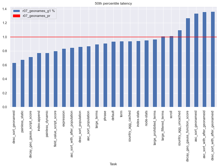
As we can see, the G1 GC is generally faster than the parallel GC, up to 40% faster than the parallel at best, but in some cases can be over 30% worse. Let's examine some of these cases in detail.

For all of the challenges with sort in the name, the challenge selected all documents in the index and sorted them differently. These results vary greatly between the GC algorithms, which highlights the importance of comparing the algorithms on your particular workload. In particular notice the desc_sort_with_geonames and asc_sort_with_geonames challenges, which together represent the best improvement and almost the worst penalty, solely by changing the order of the sorting.

Also notice on the painless_* , *_script_score, and expression challenges. These all use Elasticsearch script_score to rank results, and all perform better under the G1 GC. Compare that with the decay_gauss_function_score, which uses the native gauss function to score, and performs faster under the parallel GC. This of course has to do with the amount of objects being created on the heap, and their size, during each type of operations. Each use-case has it's own behaviors and patterns, so the GC algorithm in use should match the behavior patterns of your clusters.

Some operations in Elasticsearch (say, aggregation queries) require much fewer objects in the heap than other operations (say, script queries). The more heap-based operations your cluster will be running, the more important it is to test with different GC algorithms to see which one performs better.

Closing

The main takeaway from our benchmarks is that the G1 GC is generally a good choice, but in some workloads can actually perform worse than the parallel GC.

Like before, the benchmark shown here is just in order to make a point. Obviously for any real workload you'll be using a larger machine for your data node.

Another thing to note is the tight correlation between the total memory the machine has, the heap size used, and the GC algorithm selected. Changing one will affect the others, so you should run the benchmarks with a couple of permutations to find out the ideal combination.

Our team specializes in taking detailed measurements of your production workload and creating benchmarks specifically tailored to your environment. We have done it many times before, and for every customer we ran this benchmark we found a different sweet-spot because of different use-cases, usage patterns, and data shapes and sizes.

Run similar benchmarks for your environment, pay for it a bit upfront, and that'd save you costs and headaches later down the road, granted.