
 Jeovanny Alvarez
Elasticsearch Aggregations are working units that help build analytical data across a set of documents. This guide will help you get started and optimize your ops.
When it comes to Elasticsearch, aggregations play a huge role. But what are Elasticsearch Aggregations all about? Here is a thorough guide to get you up to date with everything you need to know about Aggregations, and how to use this feature effectively for smooth and sustainable results.
What is an Elasticsearch Aggregation?
An aggregation in Elasticsearch is a mechanism that allows you to generate metrics, statistics, or other analytics about the data contained in your indices. An aggregation is a function that can be applied to a data set to compute a result. Aggregations allow you to group like documents according to whatever parameters you wish. You can think of aggregations as buckets of data that you can slice and dice in many different ways.
Aggregations let you perform computations over document data, making it easy to get the insights you need. They can be used to answer questions such as:
- What are the top five selling products on our website?
- How many tweets were sent in the past hour?
- What is the average sale price for a product in our inventory?
Aggregations are often used to better understand data. In fact, they are used very heavily when generating visualizations in Kibana. If you create a pie chart visualization based on the value of a field for example, Elasticsearch will use an aggregation to split the documents into buckets based on the defined criteria and then Kibana will use the results of that aggregation to create the visualization.
The Prerequisites
Before you actually start using Elasticsearch aggregations, there are few steps you’ll need to take. For starters, you should have a fully functional ELK setup. The ELK stack is essentially an open source analytics solution that helps with log management. It harvests, processes, and stores data from multiple sources, something that becomes extremely important as you start scaling up fast.
Elasticsearch 7.x comes bundled with Java and it is pretty straightforward to set up. A real memory circuit breaker helps improve performance and you also get a 1-shard policy. It also has a new cluster coordination layer to improve scalability.
In addition to a working ELK setup, you’ll also need a schema (or data) within your Elasticsearch index. For example, this can be the data that has been uploaded via the Kibana UI log file. The aggregation syntax is another crucial component.
Here’s the basic structure of the Elasticsearch aggregation syntax:
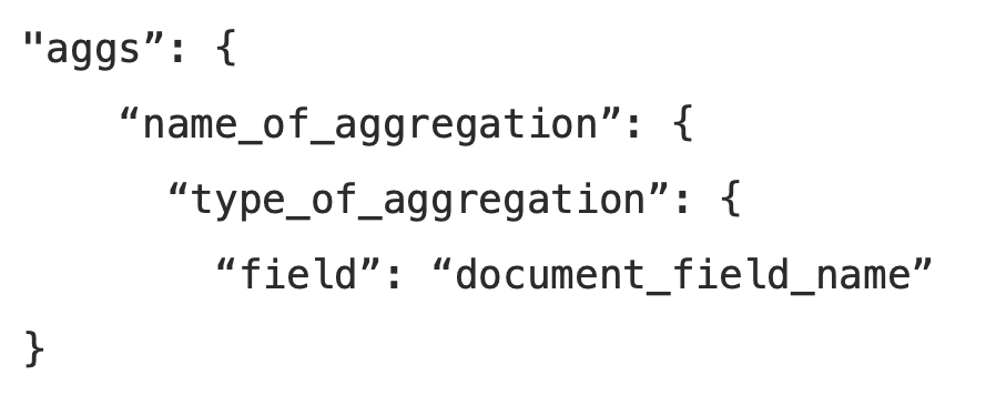
- Aggs - This keyword basically indicates the use of an aggregation.
- Name_of_aggregation - The name of aggregation defined by the user.
- Type_of_aggregation - This shows the type of aggregation that’s being used.
- Field - The field keyword is used to define the exact field that will be used
- Document_field_name - The column name of the targeted document.
Types of ElasticSearch Aggregations
There are many different types of Elasticsearch aggregations, but in general, they can be grouped into three main categories:
- Bucket aggregations: Bucket aggregations create groupings or buckets of data. For example, you can use a date range aggregation to put documents into distinct buckets based on their event end date. You can have a bucket for all documents where the end date is in less than a week, another where it is less than 30 days from now but also older than 1 week from now, and finally a 3rd bucket that has all documents that have an end date greater than 30 days from now. Bucket aggregations are often used to find patterns in data or for analytical purposes to simply find a grouping of like documents.
- Metric aggregations: Metric aggregations calculate a statistic or value from a set of documents. Using the built in functions, you can calculate the average, min, max, cardinality, etc. If you need a more complex calculation, you can use Painless scripting to generate the value you need.
- Pipeline aggregations: Pipeline aggregations are special in that they work on the outputs produced from other aggregations rather than data contained within the documents. They work using a special ‘buckets_path’ parameter that tells the location within the parent or sibling aggregation where it can find the value it should use for calculations.
Some examples for Elasticsearch aggregations and how they are categorized:
- Terms Elasticsearch aggregation - You can use this bucket aggregation to generate buckets with the help of field values, one bucket per unique value.
- Cardinality Elasticsearch aggregation - When it comes to finding the count of unique values in specific fields, this metric aggregation is what you need.
- Stats Elasticsearch aggregation - The metric aggregation to use to quickly get min, max, ave, etc.
- Filter Elasticsearch aggregation - Looking to filter various documents into a single bucket for calculating metrics? This is the aggregation you need, to be placed under any bucket aggregation.
Aggregation syntax in Elasticsearch / OpenSearch
Aggregations in Elasticsearch can be utilized in conjunction with the Query DSL for searches. You can first specify any query to limit the result set that you aggregate on or you can omit the query entirely (which essentially acts like a ‘match_all’ query in that the aggregations will act on all documents within the specified indices). Next you can begin to define your aggregations.
Each aggregation in Elasticsearch generally has its own specific syntax that is explained quite well within the Elasticsearch online documentation. In general though, an aggregation begins with the ‘aggs’ or ‘aggregations’ key. Each aggregation is first named (which can be any valid string), which is then followed by the type of aggregation, and then finally the parameters of the aggregation.
In addition, aggregations can be multi-layered and have sub-aggregations, similar in structure to nested fields. This is a very useful feature that will be shown in some examples in the sections below.
How to Use Elasticsearch Aggregations?
The three commonly used aggregation types are bucket, metric and pipeline aggregations. Here is a walkthrough of how they work.
Bucket Aggregations
Bucket aggregations are a way of grouping documents together in Elasticsearch. They are similar to the group-by feature in SQL, but work on a per-field basis. This makes them particularly useful for aggregating data from multiple sources, such as logs from multiple servers.
Some of the more commonly used bucket aggregations include the ‘terms’, ‘date range’ (or date histogram), and ‘geo-distance’ aggregations:
- The terms aggregation allows you to split documents into buckets based on the available terms of a field. For example, if you have a field named ‘make’ for a vehicle index, it can split the documents into buckets for ‘Ford’, ‘Chevy’, ‘Tesla’, etc. It is useful for fields that have distinct categorizations that are shared across the documents. It is not very useful for fields with any number of arbitrary values like a ‘description’ field that is unique to every document in the index.
- The ‘date range’ and ‘date histogram’ aggregations allows you to organize your documents based on specific date/time intervals. This is very useful in gathering analytics allowing you to see and compare how your data changes over time. For example, you can use a date histogram aggregation to segment your data based on the calendar month. These aggregations are typically used in conjunction with other sub-aggregations to gain even more insight into your data. For example, after segmenting your data by calendar month using the date histogram, you can follow it up with a ‘sum’ metrics aggregation that sums up the sales giving you a month by month sale comparison.
- The ‘geo-distance’ aggregation allows you to group your documents based on proximity to a certain geo point. For example, you can group all results that are within 1 mi from the specified point, followed by another grouping of results that are within 1-10 mi from the specified point, followed by a final grouping for all other results greater than 10 mi from the specified point.
These are just a few of the 30+ bucket aggregations available to use. While bucket aggregations are powerful on their own, they tend to be more useful when used in conjunction with the other aggregation types.
Metrics aggregations
Metric aggregations in Elasticsearch let you calculate statistics or metrics, such as a sum or percentile from field values. To calculate a metric aggregation, you specify the name of your aggregation, the type of metric, and the field you wish to run the calculation on. For example, the following shows how to create an aggregation named price_max that finds the max value of the purchase_price field. This is useful if you want to find the highest price of an item in your inventory for this example.
 {
    "aggs":{
      "price_max":{
          "metric":"max",
          "field":"purchase_price"
      }
    }
 }
Most metric aggregations calculate a single metric or statistic. The stats aggregation is different in that it calculates multiple metrics at the same time including ‘min’, ‘max’, ‘sum’, ‘count’ and ‘avg’. This can be a real time saver as it allows you to do multiple calculations with a single request.
Besides these straight-forward aggregations that calculate a value, there is one metrics aggregation in particular worth pointing out. It is called the ‘Top hits’ aggregation. This one can be particularly useful as it can even be used in certain searching scenarios. It is used in a sub-aggregation context, meaning there should be a top-level aggregation above it. The purpose of this aggregation is to display the ‘top hits’ from the parent aggregation. In the example above for the max purchase price, you can use a ‘top_hits’ sub-aggregation to return the item that has the highest price so you can get additional information about it.
Using top_hits in a search scenario is useful for group_by types of searches where you group your result set based on certain criteria. Take the following query for example that searches across the same vehicles index used in examples above.
POST vehicles/_search?size=0
{
  "query": {
    "multi_match": {
      "query": "new 4 door sedan",
      "fields": [
        "make",
        "model",
        "type",
        "description"
      ]
    }
  },
  "aggs": {
    "make": {
      "terms": {
        "field": "make",
        "size": 10
      },
      "aggs": {
        "hits": {
          "top_hits": {
            "size": 10
          }
        }
      }
    }
  }
}
This query will search across the vehicles index within the listed fields in the multi-match query using the given query text. It returns 0 hits from the search and instead returns the top 10 hits for matches within the aggregations. The aggregations will separate out your result set so that matches for each vehicle make will be contained within their own respective buckets. If your website displays the results separated by make, it is then much easier for your developers to use the provided JSON as-is without requiring additional parsing logic. The following is an example of the results set of this query:
{
  "took" : 1,
  "timed_out" : false,
  "_shards" : {
    "total" : 1,
    "successful" : 1,
    "skipped" : 0,
    "failed" : 0
  },
  "hits" : {
    "total" : {
      "value" : 220,
      "relation" : "eq"
    },
    "max_score" : null,
    "hits" : [ ]
  },
  "aggregations" : {
    "Category" : {
      "doc_count_error_upper_bound" : 0,
      "sum_other_doc_count" : 0,
      "buckets" : [
        {
          "key" : "Ford",
          "doc_count" : 101,
          "docs" : {
            "hits" : {
              "total" : {
                "value" : 8,
                "relation" : "eq"
              },
              "max_score" : null,
              "hits": [ ... ]
            }
          }
        },
        {
          "key": "Kia",
          "doc_count": 89,
          "docs": {
            "hits": {
              "total": {
                "value": 8,
                "relation": "eq"
              },
              "max_score": null,
              "hits": [ ... ]
            }
          }
        },
        {
          "key": "Tesla",
          "doc_count": 10,
          "docs": {
            "hits": {
              "total": {
                "value": 8,
                "relation": "eq"
              },
              "max_score": null,
              "hits": [ ... ]
            }
          }
        },
        ...
      ]
    }
  }
}
Note the size=0 parameter of this query. This is an important query enhancement for a lot of aggregation queries. In most cases when you run aggregation queries, you don’t care about the hits from the search query and instead are only interested in the results of the aggregations. By setting the size to 0 you can lower the payload size and allow for more efficient caching (See aggregation caches here).
Pipeline Aggregations
One of the things that makes pipeline aggregations so powerful is that they allow you to do more complex aggregations by chaining a sequence of simple aggregations together. For example, you could compute the average of a set of numbers and then use that average as input to a second aggregation that computes the standard deviation.
The pipeline aggregations have a unique syntax for the special buckets_path field. The Elastic documentation defines this syntax as:
AGG_SEPARATOR       =  `>` ;
METRIC_SEPARATOR    =  `.` ;
AGG_NAME            =  <the name of the aggregation> ;
METRIC              =  <the name of the metric (in case of multi-value metrics aggregation)> ;
MULTIBUCKET_KEY     =  `[<KEY_NAME>]`
PATH                =  <AGG_NAME><MULTIBUCKET_KEY>? (<AGG_SEPARATOR>, <AGG_NAME> )* ( <METRIC_SEPARATOR>, <METRIC> ) ;
Essentially this syntax allows you to define a pointer to where in the aggregation hierarchy the value you wish to use for the pipeline aggregation exists. I will show some examples of how to use this syntax in the section below.
The simplest pipeline aggregation is a sequence of two aggregations, with the first aggregation computed on the input documents and the second aggregation computed on the output of the first aggregation. They can get very complex depending on the number of aggregations and aggregation depth, but here is a fairly simple example using a bucket_script pipeline aggregation that calculates the percentage of total sales per vehicle make that each model contributes to (e.g. ford mustang accounts for x% of all ford sales across all models):
POST vehicles/_search?size=0
{
  "query": {
    "bool": {
      "filter": [
        {
          "term": {
            "isSold": true
          }
        }
      ]
    }
  },
  "aggs": {
    "make": {
      "terms": {
        "field": "make",
        "size": 10
      },
      "aggs": {
        "total_sales": {
          "sum": {
            "field": "salePrice"
          }
        },
        "model_sales": {
          "models": {
            "terms": {
              "field": "model",
              "size": 10
            }
          },
          "aggs": {
            "sales": {
              "sum": {
                "field": "salePrice"
              }
            }
          }
        },
        "sales_percentage": {
          "bucket_script": {
            "buckets_path": {
              "modelSales": "model_sales>sales",
              "totalSales": "total_sales"
            },
            "script": "params.modelSales / params.totalSales * 100"
          }
        }
      }
    }
  }
}
Pipeline aggregations in Elasticsearch allow for additional insights beyond what the bucket and metrics aggregations can provide on their own. The ability to chain aggregation results together opens a whole new world of analytical insights.
Where to from here?
While aggregations in Elasticsearch are powerful mechanisms for better understanding your data, you do need to take care when using them. Some aggregations can be very expensive and other factors such as using deep levels of sub-aggregations, the size of the data set that is aggregated on, etc. can cause aggregations to consume a lot of machine resources.
This is also where Pulse, our comprehensive monitoring suite, can save your team time and reduce your ongoing maintenance costs. We are world-class experts, supporting both Elasticsearch and OpenSearch in just about every aspect imaginable. Our platform can give you intelligent alerts driven by machine learning and actionable insights for things that matter. So schedule a demo today and let us help you write, monitor and/or maintain your aggregations with ease.


Comments (1)
Some info about aggregation accuracy and how to control it would make the guide even more comprehensive.
Comments are now closed