
 Cláudio Lemos
How to optimize search results ranking on Elasticsearch and OpenSearch - from the very first steps to the more advanced features it offers.
Elasticsearch (ES) has been dominating the backend of text search apps that are built for heavy usage and top performance. It’s a text-based search engine database that allows you to index, search, and analyze vast volumes of documents within seconds. The near real-time response is achievable by leveraging a unique indexing algorithm that in addition allows distribution across multiple machines and clusters, to support search at scale.
However, performance in terms of query speed and latency is not the only thing you want to have optimized when working with search engine software like Elasticsearch. Retrieving and correctly ranking the relevant documents is a challenge by itself, one that's often viewed as a tradeoff between how fast the results are returned and what’s their relevancy. ES has multiple techniques to improve search relevance ranking, including built in ML features. In this blog post, I’ll demonstrate how you can set up a cluster and apply some methods to control the relevance of the results.
This post is written in collaboration with TensorOps and it is the first in a series. We collaborate with their unique ML offering to introduce ML to search platforms, including ElasticSearch and OpenSearch and beyond.
We are going to discuss Elasticsearch, but all content and advice applies to OpenSearch as well - a recent fork of Elasticsearch by Amazon.
This is by no means a comprehensive list of ways to improve search relevance, also referred to as Search Relevance Engineering. It’s just setting the scene to get you going, and there is a lot more that could be done. Some of those additional approaches and methods will be discussed in future posts.
I’ll accompany this post with a step-by-step tutorial in Python so you can follow along. Let’s start.
Setting up your environment
If you don’t have an Elasticsearch cluster available to play around with, it’s easy to run one locally via Docker:
docker run --name es01 --net elastic -p 9200:9200 -it docker.elastic.co/elasticsearch/elasticsearch:8.6.2
Then make sure your Python environment is all set up. You’ll start off by installing and importing the libraries you will need for this project. In this case you’ll be using elasticsearch and elasticsearch-dsl.
pip -qq install elasticsearch
pip -qq install elasticsearch_dsl
Now you are ready to init your Python code and set up the ES client:
from elasticsearch import Elasticsearch
from elasticsearch_dsl import Search, Q

es = Elasticsearch('http://localhost:9200/')
es.info()
Congratulations, you’ve set up Elasticsearch! If everything is working correctly, you’ll be seeing the message ‘You Know, for Search’ as the output upon running es.info().
Loading sample data
You’ll now need some data to index on the search engine. You will be using a movie database from Kaggle. After downloading the file, add it to your project’s data folder and import it. For quicker indexing, you’ll only be sampling 5000 rows. import pandas as pd
df = pd.read_csv('/data/movies.csv').dropna().sample(5000).reset_index()
The rows include information for each movie such as plot, cast, release year. So you’ll need to include the proper schema on the mappings field when creating the index.
mappings = {
        "properties": {
            "title": {"type": "text", "analyzer": "english"},
            "ethnicity": {"type": "text", "analyzer": "standard"},
            "director": {"type": "text", "analyzer": "standard"},
            "cast": {"type": "text", "analyzer": "standard"},
            "genre": {"type": "text", "analyzer": "standard"},
            "plot": {"type": "text", "analyzer": "english"},
            "year": {"type": "integer"},
            "wiki_page": {"type": "keyword"}
    }
}

es.indices.create(index="movies", mappings=mappings)
Now that you have everything prepared, you can send the data to be indexed in bulk.
from elasticsearch.helpers import bulk

bulk_data = []

for i, row in df.iterrows():
    bulk_data.append(
        {
            "_index": "movies",
            "_id": i,
            "_source": {
                "title": row["Title"],
                "ethnicity": row["Origin/Ethnicity"],
                "director": row["Director"],
                "cast": row["Cast"],
                "genre": row["Genre"],
                "plot": row["Plot"],
                "year": row["Release Year"],
                "wiki_page": row["Wiki Page"],
            }
        }
    )

bulk(es, bulk_data)
Tweaking search results rankings
After setting up the cluster with some data, let's look closely at how Elasticsearch ranks search results.
Text relevance is one of the most important factors that influence Elasticsearch search results rankings. In other words, this is the order of results returned by Elasticsearch for a given query. Elasticsearch uses a combination of text matching and scoring algorithms to determine the relevance of search results. The text matching algorithm checks if the search query terms appear in the document's fields, such as title, description, or content. The scoring algorithm then assigns a score to each document based on how well it matches the query terms. The document with the highest score ranks first in the search results.
Everything in that respect is configurable, and there is hardly any use-case where you want to keep the default settings. Let’s dive into the details of the more prominent parts that make up a usual search relevant engineering process, and look into each component, or layer, individually. This is by no means a comprehensive guide, but a solid first step for you to follow and continue from.
Layer 1: Scoring with BM25
TF/IDF (Term Frequency/Inverse Document Frequency) is a traditional ranking algorithm that assigns a weight to each term in a document based on its frequency in the document and its rarity in the corpus. The weight of each term is calculated by multiplying its term frequency (TF) by its inverse document frequency (IDF). The resulting weight is used to rank the documents based on their relevance to the search query.
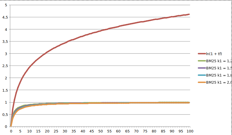
BM25 (Best Matching 25) is a more advanced ranking algorithm that takes the length of the document and the average length of documents in the corpus into account. BM25 also uses a saturation function to prevent the weight of a term from growing too large. BM25 has been shown to outperform TF/IDF in many cases, particularly with longer documents.
There are several important differences between tf/idf and BM25. In general, if the documents in your corpus are short and you are looking for a simple ranking algorithm, TF/IDF may be a good choice. However, if your documents are longer and more complex, or if you are looking for a more advanced ranking algorithm, BM25 may be a better option.
BM25 is considered to be an improved version of tf/idf, and thus for a few years now it’s the default option used by Elasticsearch for scoring. For this example, you will implement a search query using default Elasticsearch configurations, which means BM-25 will be used as the base ranking algorithm. You can start off by creating a new index:
es.indices.create(index="movies-bm25")
movies_idx.put_mapping(
    body={
        "properties" : {
            "title": {"type": "text", "analyzer": "english"},
            "ethnicity": {"type": "text", "analyzer": "standard"},
            "director": {"type": "text", "analyzer": "standard"},
            "cast": {"type": "text", "analyzer": "standard"},
            "genre": {"type": "text", "analyzer": "standard"},
            "plot": {"type": "text", "analyzer": "english"},
            "year": {"type": "integer"},
            "wiki_page": {"type": "keyword"}
        }
    }
)
You can change the default settings of the BM25 algorithm that’s being used. This is an advanced configuration that requires some testing as to the actual numbers to use, but just to demonstrate how it’s done. Notice how we create a new similarity settings, and then use it explicitly in the mapping:
movies_idx.put_settings(
    body={
        "similarity":{
            "bm25-example": {
                "type": "BM25",
                "k1": 2, # controls non-linear term frequency normalization (saturation) - default is 1.2
                "b": 0.5, # controls to what degree document length normalizes tf values - default is 0.75
                "discount_overlaps": True, # determines whether overlap tokens are ignored when computing norm
            }
        }
    }
)

movies_idx.put_mapping(
    body={
        "properties" : {
            "title": {"type": "text", "analyzer": "english", "similarity": "bm25-example"},
            "ethnicity": {"type": "text", "analyzer": "standard"},
            "director": {"type": "text", "analyzer": "standard"},
            "cast": {"type": "text", "analyzer": "standard"},
            "genre": {"type": "text", "analyzer": "standard"},
            "plot": {"type": "text", "analyzer": "english", "similarity": "bm25-example"},
            "year": {"type": "integer"},
            "wiki_page": {"type": "keyword"}
        }
    }
)
With the new settings applied, reindex the data from the original index to the new one:
es.reindex({
    "source": {
        "index": "movies",
    },
    "dest": {
        "index": "movies-bm25"
    }
})
The movies index will use the standard BM25 configurations, while movies-bm25 will use our custom BM25 configurations. For comparison, you can perform the same query on both indexes. In this case, let’s use the word wedding.
es.search(
    index="movies-bm25", # repeat for "movies"
    query={
        "bool": {
            "must": {
                "match_phrase": {
                    "title": "wedding",
                }
            },
        },
    },
    _source={
        "includes": [ "title" ]
    }
)
For this query, Big Wedding, “The Big Wedding” jumped to the top on the BM-25 index, while on the original it wasn’t even showing up in the Top 3.
Layer 2: Field Boosting
Elasticsearch allows you to make individual fields automatically count more towards the relevance score at query time. That is possible by using the boost parameter. For this example, you will boost the title by making it twice as important as the other fields.
Let’s test it out:
es.search(
    index="movies-boost",
    query={
        "query_string": {
            "query": "girl",
	“fields”: [“title^2”]
        },
    }
)
As expected, the first result The Girl in the Park got twice the score it achieved on the original index.
It’s also possible to set boosts on the index level via the index mappings, but I don’t recommend that. Use query-time mappings which gives you more flexibility and no need to reindex every time you want to change boost parameters.
The actual boosts to use, however, are just magic numbers. There’s no “right” and “wrong” here. Just test this carefully until you land on a satisfactory configuration.
Layer 3: Adjusting with Function Score
The function_score query allows you to modify the score of documents that are retrieved by a query. This is useful in cases where the score function is computationally expensive and it is sufficient to compute the score on a filtered set of documents.
You can combine several functions which can optionally choose to apply the function only if a document matches a given filtering query.
es.search(
    index="movies",
    query={
    "function_score": {
      "query": { "match_all": {} },
      "boost": "5",
      "functions": [
        {
          "filter": { "match": { "year": "1996" } },
          "random_score": {},
          "weight": 30
        },
        {
          "filter": { "match": { "year": "1994" } },
          "random_score": {},
          "weight": 50
        }
      ],
      "max_boost": 50,
      "score_mode": "max",
      "boost_mode": "multiply",
      "min_score": 50
    }
  },
    _source={
        "includes": [ "title", "year" ]
    }
)
Layer 4: Synonyms
Synonyms are words or phrases that have the same or similar meanings. For example, "car" and "automobile" are synonyms because they refer to the same thing. Synonyms can also be words that are related to each other in some way, such as "dog" and "pet". We usually call this an “umbrella synonym” to indicate it’s not bidirectional - a dog is a pet, but a pet isn’t necessarily a dog.
In Elasticsearch, synonyms are used to expand search queries and improve the relevance of search results. When a user enters a search query, Elasticsearch looks for matches in the index based on the query’s terms. If the search query contains a synonym, Elasticsearch will also look for matches based on the synonym.
For example, if a user searches for "automobile", Elasticsearch will also look for matches that contain the word "car". This is because "car" is a synonym for "automobile". By expanding the search query to include synonyms, Elasticsearch can deliver more relevant search results to users.
To use synonyms in Elasticsearch, you need to create a list of synonyms and add them to the index. This can be done using the Synonym Token Filter, which is a built-in feature of Elasticsearch.
To create a list of synonyms, you can use a text editor or a spreadsheet program. Each line in the list should contain a synonym group, with each synonym separated by a comma. For example:
car, automobile, vehicle
dog, pet, animal
Once you have created the list of synonyms, you can add it to the index by creating a custom analyzer that includes the Synonym Token Filter. You can then apply the analyzer to the fields in the index where you want to use synonyms.
Synonyms can be set on either index time (so the index contains the expanded terms), or on search time only (so index is not bloated but more search time work is needed), or both. It’s usually easier to maintain synonyms on search time but it’s not without a cost.
Using synonyms in Elasticsearch can help improve the relevance of search results by expanding the search query to include related terms. This can help users find what they are looking for more quickly and easily.
But you need to tread carefully. While synonyms usually improve recall by finding relevant documents that otherwise wouldn’t be found, overusing synonyms can impact precision negatively. That is why synonyms are usually used in conjunction with field boosting and other aforementioned methods to limit its effect.
Conclusion
As clearly evident, a multi-layered approach to search relevance engineering is what separates great Elasticsearch clusters from the good ones. That said, you also need to watch out and refrain from over-engineering them because the results can be counterproductive and hamper your accuracy. Stay tuned for the next article in a series that will cover the key aspects of ML-based search and relevance, showing how to take search relevance in Elasticsearch to the next level.


Comments are now closed