 Shai Greenberg
In this post, we will explore Presto's Geospatial capabilities, and leverage Presto's Geospatial function to enrich data and get geographical insights.
In the previous post we've seen how to use Presto to explore our data and store it on S3. In this post we'll explore a different feature of Presto - the Geospatial functions. Some example use cases would be finding out distances between geographical points of interest, finding out which points are closest to a single point, or using connections between points and even shapes to provide insights on data and enrich it. We'll explore all of that in this post, following a brief discussion on the appropriate geo-data format for use with Presto.
Understanding the required data format
To allow geospatial functions, Presto needs the data (or a transformation of the data) to be of specific types and format. The basic format we'll be working with is WKT - Well-Known Text. In that format, a geometric data point looks like this:
POINT (x y)However, data points are not the only types of geometric entities available. For instance, the polygon and the multipolygon allow us to have shapes as a data type, thus associating them with a row of data. What purpose does that serve? Well, consider that data entires may represent more than a specific point on a map - a building, a city, or a path.
LINESTRING (0 0, 1 1, 1 2)
POLYGON ((0 0, 4 0, 4 4, 0 4, 0 0), (1 1, 2 1, 2 2, 1 2, 1 1))
MULTIPOINT (0 0, 1 2)
MULTILINESTRING ((0 0, 1 1, 1 2), (2 3, 3 2, 5 4))
MULTIPOLYGON (((0 0, 4 0, 4 4, 0 4, 0 0), (1 1, 2 1, 2 2, 1 2, 1 1)), ((-1 -1, -1 -2, -2 -2, -2 -1, -1 -1)))
GEOMETRYCOLLECTION (POINT(2 3), LINESTRING (2 3, 3 4))
Notice that I've used the word "geometric" rather than "geographical" or "geospatial" to describe those types, since indeed they refer to shapes on a map, and do not describe the real-world semantics of such points. So, in the context of getting actual distances between points, we'll first need to convert them to geospatial form. We'll get to how to do this later, but first, we have to get our data into the WKT format in the first place.
Finding the relation that contains a point
In the previous post, we've found the locations of recycling containers in Israel. Now we'd like to find out which municipality each container is in. OpenStreetMap doesn't actually contain that information: instead, it contains relations that describe the boundaries of municipality. So to understand which municipality a data point is in, we need to try and pinpoint which relation of the appropriate type it is in. Now you might be starting to connect the dots: the Geospatial functions allow you to do just that, but you'll first have to get the point data and the municipality data in the WKT format.
Getting the data into the WKT format: As the point data is the easy part, we'll start with the municipality data. We already have access to OpenStreetMap via Presto established the previous post, so it's tempting to try and use Presto to assemble the WKT data from the municipality relations, but this is a bit out of scope at this point. We'll leave that as an exercise, and instead use some existing services and a little code to get the job done.
I found Overpass-turbo to be a sufficient way to extract the relevant data for this post, although there are other possible ways to achieve the same result. Overpass-turbo allows exporting a selection from OpenStreetMap in several formats. Specifically, one can extract a GeoJSON file with the information requested, which can then be converted easily into WKT.
The information we require is the municipality boundaries for Israel. According to the OpenStreetMap WIKI, this can be found by querying admin_level=8 within Israel. To do that, just focus the map in the site on the relevant geography, and then paste the query:
[out:json][timeout:25];
(
  // query part for: “admin_level=8”
  relation["admin_level"="8"]["boundary"="administrative"]({{bbox}});
);
  out body;
>;
out skel qt;
You can then click "Export" to export the data, and choose the GeoJSON format.
We'll convert it to WKT using a python script. The relevant code can be found here. I won't go into too much detail about the script - generally, what it does is:
1) filter the data to return only municipalities for which we have polygon data, rather than point data.
2) Create records with the english name of the municipality and the geometric shape in WKT format
3) Store those records in a Parquet file in S3
You'll note that this is not a complete list of Israeli municipalities, so we're bound to have missing data here and there.
Using Presto to query the data: For this part, you'll want to change the references to the S3 buckets to those of your own S3 buckets.
Now that we have the data in S3, we can create a table for it in Presto.
CREATE TABLE glue."bdbq-osmplanet".boundaries (
    name varchar,
    coordinates varchar
 )
 WITH (
    external_location = 's3://bdbq-israel-boundaries/parquet/',
    format = 'PARQUET'
 )
We can now take this table and the recycling containers table created in the previous blog, and join them, using the geospatial function ST_Contains to match the data point with the relevant municipality:
SELECT * FROM glue."bdbq-osmplanet".containers
CROSS JOIN glue."bdbq-osmplanet".boundaries AS b
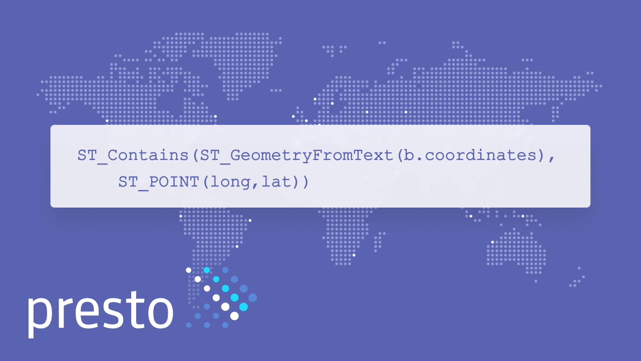
WHERE ST_Contains(ST_GeometryFromText(b.coordinates),ST_POINT(lat,long))And... get no results. What went wrong?
Well, as it turns out, the proper format to use with geospatial functions is (long,lat) rather than (lat,long). While this has no direct impact on geometric functions, we didn't get a match since the data extracted from the municipalities is in one format, and the created point in another. To solve that, the correct query has the coordinates in the reverse order:
SELECT * FROM glue."bdbq-osmplanet".containers
  CROSS JOIN glue."bdbq-osmplanet".boundaries AS b
WHERE ST_Contains(ST_GeometryFromText(b.coordinates),ST_POINT(long,lat))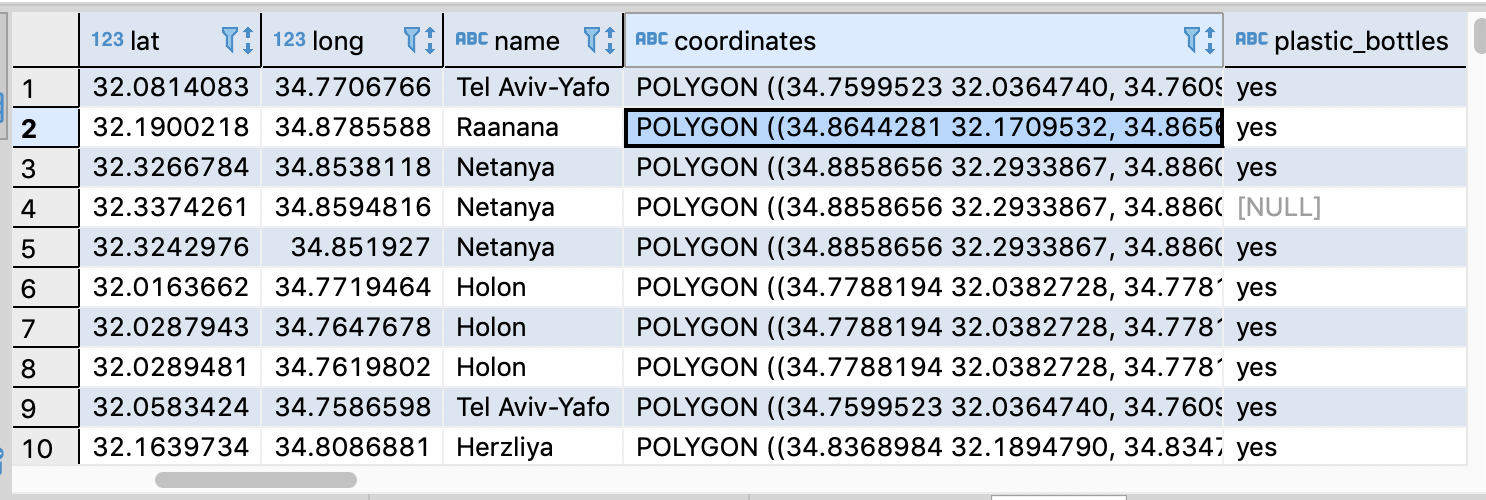
Awesome, we now have the municipality data for each container. You can do a lot more with that data in hand, such as find out how many containers are in each municipality, but our focus here is the geospatial functions, so let's explore another one.
Finding out which points are closest to a single point
For our next geospatial feat, we're going to help a truck driver from a bakery in Israel determine exactly where he's at.
A popular use case for geospatial queries is "what's nearby" - you've probably tried asking applications in your mobile phone that very question, and you may have even asked people once or twice. Truck drivers normally have pre-determined routes: at the very least they know which places (such as a convenience store) they should visit within a certain time period. However, once they're actually within the store, there's an advantage to knowing exactly which one they're at: A driver searching through an application find the current store's delivery details may accidentally choose the wrong store. Being able to pinpoint a coordinate and determine the closest store would save time and increase efficiency.
Getting the stores data: we'll first have to create an additional table that contains all of the shops the driver might find himself in.
As metadata in OpenStreetMap is often region-dependent, we'll need to read up on the relevant tags and do some exploratory analysis in order to find out the correct query. Since we've already done similar things in the previous post, I'll skip the details this time around. The eventual query would look something like this:
CREATE TABLE glue."bdbq-osmplanet".supermarkets_il
 WITH (
     external_location = 's3://bdbq-osmplanet/supermarkets_il',
     format = 'ORC')
 AS (SELECT *
FROM glue.osm.osmplanet
WHERE lat BETWEEN 29.5013261988 AND 34.2654333839
 AND long BETWEEN 33.2774264593 AND 35.8363969256
 AND element_at(tags, 'shop') IN ('supermarket','convenience'));
Notice that we're still using lat and long to determine "what's in Israel", although by now you should know you have a more accurate way to do that using a geospatial function. That kind of function would take a longer time to run - after all, rather than working directly with the coordinate fields, it would run a transformation on them. However, it would produce more accurate results. As the details have already been discussed, this is also left as an exercise.
Calculating which stores are closest to a single point: Once we've created the table, we can query it. Let's say the driver is at a coordinate near Rabin Square. To use the geospatial distance function, we need to convert the geometric points into spherical geography:
SELECT *,distance FROM
  (SELECT element_at(tags,'name:en'),*,ST_DISTANCE(
   to_spherical_geography(
   ST_POINT(long,lat)),to_spherical_geography(ST_POINT(34.780572,32.080883))) as distance
 FROM  glue."bdbq-osmplanet".supermarkets_il) AS b
 WHERE distance < 200
 ORDER BY b.distance ASC;
This query first calculates the stores' distance and then sorts the stores based on that distance, to return the closest ones. Based on the coordinate given, we can say that the driver is probably in one of returned stores (assuming of course OpenStreetMap is updated with the relevant ones).
There's obviously a lot more to explore here as well - the use of distance can be extended to more complex analysis use cases such as finding the distance between shops and the closest ATM. Presto also supports Bing Tiles, which allows determining the existence of points within a zoomable tile. However, rather than delve deeper into geospatial functions - as you've been taking an interest in our Presto series, we'd love to hear your input on what you'd like us to cover in a future post.


Comments are now closed